In the Great Lakes, harmful algal blooms (HABs) are dominated by cyanobacteria, commonly called blue-green algae, that grow rapidly when conditions warrant (warm water temperatures and excess nutrients). Cyanobacteria are ancient organisms that have been producing oxygen through photosynthesis for billions of years, helping shape Earth’s atmosphere. Today, these blooms can form dense surface scums and sometimes produce toxins that pose risks to people, pets, wildlife, and drinking water supplies.

HABs primarily occur in several areas across the Great Lakes, including western Lake Erie, Saginaw Bay in Lake Huron, and Green Bay in Lake Michigan. They reduce water clarity, disrupt recreational activities, and affect local ecosystems. While HABs are a concern throughout the region, western Lake Erie experiences some of the largest and most intense cyanobacterial blooms, making it a focal point for extensive monitoring for research and forecasting. These blooms are often dominated by the Microcystis algae, a type of cyanobacteria capable of producing toxins known as microcystins.

Each year, researchers at NOAA’s Great Lakes Environmental Research Laboratory (GLERL) and the University of Michigan’s Cooperative Institute for Great Lakes Research (CIGLR) monitor and track Great Lakes HABs using field observations and advanced technologies. Together, these efforts help scientists better understand bloom development, toxin levels, and potential impacts on communities, improving our ability to warn people about bloom conditions.

What the 2026 Lake Erie Seasonal HAB Forecast Tells Us

According to NOAA’s National Centers for Coastal Ocean Science (NCCOS) early season HAB outlook released on June 25, western Lake Erie was forecast to experience a moderate cyanobacterial harmful algal bloom (HAB) during the 2026 season (roughly July to October).

In western Lake Erie, bloom severity is largely driven by the amount of phosphorus entering the lake from the Maumee River watershed during the spring and early summer. NOAA measures bloom severity using an index that reflects the amount of cyanobacterial biomass, or blue-green algae, present during the bloom’s peak 30-day period, which generally occurs in August but can vary from year to year. A severity index between 3 and 4.5 indicates a moderate bloom, while values above 5 indicate a severe bloom. This season’s bloom was forecast to fall between 3 and 4.5, comparable to the blooms observed in 2020 and 2023 but in contrast to 2011 when extreme bloom severity reached a record-setting index of 10. Although an early April rainfall event caused phosphorus loading in western Lake Erie, bloom severity ultimately depends on weather conditions and rainfall through July.

Bloom size tells only part of the story. Because toxin levels can vary independently of bloom conditions, researchers are developing forecasts for both bloom severity and toxicity.

Tracking Harmful Algal Blooms Across the Great Lakes

Predicting the season’s bloom severity is only part of the challenge in managing impacts from HABs. Throughout the season, scientists from GLERL and CIGLR monitor bloom development, movement, and toxicity across the Great Lakes to better understand bloom dynamics, detect emerging HAB activity, and provide timely information to resource managers, water treatment operators, and the public.

From late April through October, researchers conduct regular monitoring cruises in western Lake Erie and Saginaw Bay, collecting water samples that are analyzed for indicators such as chlorophyll, phosphorus, and microcystin concentrations. Researchers also rely on a network of observations including buoys, satellite and aircraft-based remote sensing datasets, autonomous vehicles, and Environmental Sample Processors (ESPs) to track bloom conditions across the basin, including areas such as Green Bay.

Together, these observations provide near real-time information on bloom location, intensity, and toxicity. The data help scientists evaluate forecast performance, improve predictive models, and identify changes in bloom behavior as environmental conditions shift. By combining field observations with advanced monitoring technologies, researchers can provide more accurate and actionable information to support decision-making throughout the Great Lakes region. These observations are being used to develop new forecasting tools designed to predict toxin concentrations.

Recent research also demonstrated the importance of monitoring HAB conditions across areas of the lake. A study led by CIGLR and NOAA GLERL researchers examined how water from the Detroit and Maumee rivers interacts in western Lake Erie, creating distinct environmental conditions that influence bloom development. “We expected to find a gradient between the Detroit and Maumee river inflows, but I was surprised by how much the transition zones shifted from month to month and how distinct they were,” said CIGLR’s Jasmine Mancuso, lead author of the study. CIGLR researchers explain the study and its findings in a recent blog post, highlighting how observations across this gradient provide a more complete picture of the factors that shape HABs and can improve future bloom forecasts.

Forecasting Bloom Toxin Levels

As monitoring improves, researchers are working to better predict not only where blooms will occur, but also how toxin levels change. Because bloom size and toxin levels are not always closely linked, forecasting toxins has become an important area of harmful algal bloom research.

NOAA researchers have developed an experimental five-day toxin forecast system that predicts the probability of exceeding the recreational public health advisory level for microcystins in western Lake Erie. The system combines weekly measurements of microcystins with data on bloom conditions, weather, and lake circulation to estimate where and when elevated microcystin levels may occur. NOAA GLERL is currently working with partners at NCCOS to move the system into operational use, timely information about toxin risks in Lake Erie.

Testing with ten years of historical Lake Erie data shows that it performs well in identifying areas of increased toxin risk, including near drinking water intakes, within bloom-affected regions, and across the western basin. This long-term record was essential for testing the forecast across a range of toxin levels. “It is a relatively rare event for microcystin levels to exceed the public health advisory level,” said Mark Rowe, Ph.D., a research physical scientist at NOAA GLERL. “Only 3% of observations in the ten-year database exceeded that level. It was necessary to have a large database of observations, including the rare exceedances, to calibrate the statistical models that underpin the forecast, showing the value of long-term monitoring programs.”

By focusing on the likelihood of elevated toxins rather than bloom presence alone, these forecasts can help water treatment managers, public health officials, and coastal communities make informed decisions during the bloom season. A public version of the forecast is planned, providing earlier and more accurate information about potential toxin exposure.

Understanding the Health Risks of Harmful Algal Blooms

Some cyanobacteria that form harmful algal blooms produce toxins that can affect humans and animals. In Lake Erie, Microcystis blooms can produce microcystin, a toxin that affects the liver and contaminates drinking water sources when blooms occur near water intakes.

People can be exposed to HAB toxins through skin contact, accidental ingestion of contaminated water, or inhalation of water droplets and aerosols. Exposure can cause symptoms such as skin irritation, coughing, nausea, vomiting, and diarrhea, with more severe health effects possible in some cases.

Pets – particularly dogs – face an elevated risk when they swim in affected water and groom themselves after. Staying aware of local conditions and advisories can reduce exposure risks for both people and pets.

New research also shows that Lake Erie cyanobacteria blooms produce a mix of naturally occurring compounds that change over the course of the season. Instead of being dominated by a single toxin, blooms may shift through phases where different cyanobacteria compounds become more common. This variability adds another layer of complexity to understanding bloom impacts and highlights the importance of looking at all toxins when assessing potential risks. “These cyanobacteria are extraordinary chemical factories; they produce an astonishing diversity of chemical compounds, and we’re only just beginning to identify and understand them all. But there is some evidence that suggests that this mixture of compounds may affect human health in novel ways,” said Greg Dick, Ph.D., Director of CIGLR and senior author on the study. “CIGLR and GLERL scientists are partnering with colleagues around the region, including the Great Lakes Center for Freshwaters and Human Health, to better understand the impacts of blooms on human health and the risks they pose to people that live, work, and play in and near the lakes.”

Looking Ahead

Although 2026 is projected to be a moderate bloom year, conditions can change throughout the summer. GLERL and CIGLR scientists continue monitoring Lake Erie and other Great Lakes HAB blooms throughout the season, providing data for forecasts and water resource management. While western Lake Erie remains the primary focus of seasonal forecasting because of its large, recurring blooms, monitoring HABs in Saginaw Bay and Green Bay helps reduce HAB risks across the Great Lakes basin.

Together, these efforts support research, forecasting, and public health initiatives that help communities safely enjoy Great Lakes waters.

Additional Resources

• Harmful Algal Bloom Forecasting: NOAA’s National Centers for Coastal Ocean Science (NCCOS) HAB forecasts and partner-developed regional forecasts provide early warnings about bloom conditions, helping communities, managers, and public health officials prepare for potential impacts
• Lake Erie Harmful Algal Bloom Forecast: NOAA provides forecasts for seasonal blooms of cyanobacteria (blue-green algae) in Lake Erie, typically from July to October when warmer water creates favorable bloom conditions.
• Great Lakes Harmful Algal Blooms (HABs) and Hypoxia Program: A collaboration between GLERL and CIGLR scientists, uses satellite imagery, remote sensing, buoys, monitoring programs, and genetic techniques to understand and predict HABs and hypoxia across the Great Lakes. The data collected improves forecast models that help stakeholders, including drinking water managers, make informed decisions to protect ecosystem health and reduce risks associated with recreation, consumption, and water treatment.
• NOAA detects harmful toxin growing in Lake Erie earlier than past years: In 2025, NOAA detected levels of the harmful toxin, microcystin, in Lake Erie weeks earlier than it is usually detected in routine water tests.
• Cooperative Institute for Great Lakes Research (CIGLR) Harmful Algal Blooms (HABs) Program: This CIGLR resource highlights research on harmful algal blooms (HABs), including efforts to understand bloom drivers, improve monitoring and forecasting tools, and reduce impacts on Great Lakes ecosystems and communities.
• Toxic algae blooms are lasting longer in Lake Erie − why that’s a worry for people and pets: This article explores how longer-lasting harmful algal blooms in Lake Erie can increase risks for people, pets, and ecosystems, while explaining the science behind changing bloom conditions and toxin concerns.

As summer arrives and lake waters warm, researchers deploy buoys across the Great Lakes to gather vital environmental data. For over 20 years, the Great Lakes Environmental Research Laboratory (GLERL) and partners have developed and implemented these buoy systems to enhance NOAA’s observational capabilities and understanding of Great Lakes ecosystems. By gathering observations from across the Great Lakes, GLERL provides information that supports resource management decisions and promotes safe, sustainable ecosystems and communities.

A NOAA GLERL Real-Time Coastal Observation Network (ReCON) buoy in Lake Michigan.

From May through October, researchers are deploying a total of 10 buoys to collect data vital to safeguarding the millions of people who live, work, and play around the Great Lakes. Serving as a critical component of the Real-time Coastal Observation Network (ReCON), these systems stream environmental data through a wireless, internet-based system, allowing researchers to monitor lake conditions remotely without needing to be physically on the water. These platforms are strategically positioned in high-priority areas, including Western Lake Erie, Saginaw Bay and Thunder Bay National Marine Sanctuary in Lake Huron, and key coastal sites in Lake Michigan. By continuously tracking environmental conditions – such as waves, wind, water temperatures, dissolved oxygen, nutrients, and algal activity – they provide critical real-time data for safety, situational awareness, and water quality issues such as harmful algal bloom (HAB) detection, which directly informs beach closures and drinking water processing. Tracking waves and currents improves marine weather forecasts, rip current warnings, and safe navigation for commercial and recreational vessels. Beyond immediate safety risks, these observations contribute to a long-term environmental record to improve Great Lakes forecasting and ecosystem research.

“The Great Lakes buoy network monitors ecosystems to ensure environmental health, supporting vital commercial and recreational activities,” said Steve Ruberg, a research physical scientist with GLERL who specializes in observing systems research.

The success of this observational network relies on strong partnerships between federal, regional, and academic organizations. The Great Lakes Observing System (GLOS) manages the collection and public presentation of data from the buoy network, ensuring that information is readily accessible through online platforms such as its Seagull site. Most ReCON buoy data is publicly available in near-real-time for researchers, water managers, boaters, anglers, and coastal communities. The Cooperative Institute for Great Lakes Research (CIGLR) also partners with GLERL on observing systems through research, technical development, and regional coordination that keep these complex systems running. Maintaining the network requires year-round engineering, calibration, data management, and field support to ensure the systems continue delivering reliable environmental observations.

CIGLR’s role is hands-on, encompassing the engineering and maintenance of several critical platforms. CIGLR deploys and maintains GLOS-funded buoys in Little Traverse Bay and Ludington on Lake Michigan, as well as specialized ecological Synthesis, Observations and Response System (SOAR) buoys in Western Lake Erie and Saginaw Bay. These platforms are custom-tailored to the specific ecological needs of their locations. While the Lake Michigan buoys feature temperature and meteorological sensors that provide a “near-shore” look at rapidly changing conditions, the Western Lake Erie and Saginaw Bay buoys carry nutrient sensors to track HABs.

“The Western Lake Erie buoys carry nutrient sensors that inform water managers and scientists about conditions conducive to growing toxic algae,” says Russ Miller, CIGLR’s lead engineer for the buoy program. He notes that the impact extends well beyond the lab to the local economies and public safety. “The Lake Michigan buoys have temperature strings that the fishermen love… and in Ludington, tournament fishermen use the wave sensors as an objective measurement. If it’s over three feet, they know to delay. It provides an objective measurement for the community.”

Real-time and archived buoy observations help improve the reliability of Great Lakes forecasts for environmental conditions such as hypoxia (reduced oxygen levels) and HABs. Since the establishment of GLERL’s ReCON system in 2004, buoys deployed across the lakes have collected meteorological, biological, chemical, and physical observations that support monitoring and forecasting efforts. Archived at NOAA’s National Centers for Environmental Information (NCEI), these long-term datasets are used by researchers, educators, and resource managers to improve scientific models, evaluate past events, and understand changes in lake conditions over time. Data collected by buoys deployed in Lake Erie allows forecasters to predict when HAB or hypoxic water moves toward municipal water intakes, providing critical information for water management decisions.

“The observing systems established on western Lake Erie greatly enhance our environmental awareness and decision-making regarding this vital drinking water resource,” said Douglas R. Stephens, president of the Northwestern Water & Sewer District and former director of the City of Toledo Department of Public Utilities. “Access to real-time water quality data is critical for treatment decisions impacting the 500,000 citizens served by Toledo’s Collins Park Water Treatment Plant. These physical and chemical buoy observations provide background information for the continued improvement of the western Lake Erie HAB forecast, which our staff highly values for early warning of potentially toxic HAB conditions.”

This work is fundamental to the mission of GLERL to study, understand, and protect Great Lakes ecosystems and coastal communities. The GLERL Observing Systems and Ecosystem Monitoring team develops and operates technology that supports coastal environmental observation networks and advances NOAA’s ecosystem forecasting research goals, with much of this work supported by funding from the Great Lakes Restoration Initiative (GLRI), a multi-agency effort focused on protecting and restoring the Great Lakes ecosystem. Together, these observing systems provide a regional environmental intelligence network for the Great Lakes. The network of buoys is more than a collection of sensors, it is a backbone of coastal resiliency. By providing real-time insights into physical and chemical changes in the lakes, these systems help protect coastal communities, track the health of the Great Lakes, support drinking water safety, improve understanding of ecosystem conditions, and strengthen the region’s maritime economy.

Looking ahead, GLERL and partners continue to build on these observing systems by using aerial drones, autonomous surface vehicles, and real-time toxin models for harmful algal blooms. This network of buoys is far more than than a collection of sensors; it is the backbone of Great Lakes coastal resiliency.

---

Get to Know Your Buoys

The buoys highlighted below help form a coordinated Great Lakes observing network across the basin. By capturing real-time data from nearshore zones, offshore waters, and ecologically sensitive regions, these systems provide a continuous view of how the lakes are changing throughout the spring and summer seasons. Check these links throughout the season for real-time data, updates, and additional information.

Lake Michigan: Tracking Nearshore to Offshore Conditions

In Lake Michigan, multiple buoys are positioned to capture gradients from nearshore waters to deeper offshore environments.

M20 Buoy — Muskegon, Michigan

Deployed near the 20-meter depth zone, this GLERL-built and maintained system provides nearshore meteorological and water quality data that support marine forecasting and recreational safety as summer lake activity increases

Little Traverse Bay Buoy — Northern Lake Michigan

Deployed near the 20-meter depth zone, this GLERL-built and maintained system provides nearshore meteorological and water quality data that support marine forecasting and recreational safety as summer lake activity increases.

Ludington Buoy — Central Lake Michigan

This CIGLR-maintained buoy, funded by GLOS, provides wave, weather, and water condition data used by researchers and the local maritime community alike.

Lake Huron: Understanding Coastal Ecosystems and Change

In Lake Huron, deployments focus on both ecosystem monitoring and sensitive coastal environments.

Alpena Buoy — Thunder Bay National Marine Sanctuary

At the Thunder Bay National Marine Sanctuary near Alpena, this long-term monitoring buoy operated by GLERL supports ecological research and sanctuary resource management in a sensitive coastal environment.

Point Au Gres, MI Buoy — Saginaw Bay

At Point Au Gres in outer Saginaw Bay, this long-term monitoring buoy is built and maintained by GLERL and collects weather, wave, current, and water quality data in approximately 40 feet of water. These observations support ecosystem research, environmental monitoring, and forecasting efforts throughout Saginaw Bay.

SB14 & SB26 Buoys — Inner & Outer Saginaw Bay

In Saginaw Bay, two buoys co-built by GLERL and CIGLR and funded through the Ocean Acidification Program track changing water chemistry and ecosystem conditions in one of the Great Lakes’ most biologically productive regions.

Lake Erie: Monitoring Harmful Algal Blooms and Water Quality

In Lake Erie, deployments focus on high-resolution monitoring of water quality conditions that directly support harmful algal bloom forecasting and drinking water safety for surrounding communities.

WE02, WE04, WE08 Western Lake Erie SOAR Network

In western Lake Erie, the SOAR buoy network, funded through the GLRI and maintained by CIGLR, provides high-resolution observations of water quality, meteorology, and biological activity. These data are essential for monitoring and forecasting HABs and supporting drinking water safety for surrounding communities.

---

Resources

Access data from across the Great Lakes using this observational network by clicking on the resources below.

• NOAA GLERL Great Lakes Meteorological Real-Time Coastal Observation Network (ReCON): The primary Great Lakes buoy network providing real-time meteorological, physical, chemical, and biological observations used for forecasting, ecosystem monitoring, and research.
• Great Lakes Observing System (GLOS) Seagull platform: A user-friendly data portal that visualizes real-time buoy observations, lake conditions, and forecasts for researchers, resource managers, mariners, anglers, and the public.
• NOAA National Centers for Environmental Information (NCEI): NOAA’s official archive for long-term buoy datasets, supporting historical analysis, model validation, and hindcasting of Great Lakes environmental conditions.

This summer, Saginaw Bay is getting a high-tech visitor! The Great Lakes Environmental Research Laboratory (GLERL) is deploying a SeaTrac uncrewed surface vessel from July 29th to September 4th as part of the SHARC (Surface Harmful Algal Research Craft) project. SHARC is a cutting-edge effort to monitor and understand Harmful Algal Blooms (HABs) in Saginaw Bay, Lake Huron. GLERL is partnering with the National Centers for Coastal Ocean Science and the Monterey Bay Aquarium Research Institute (MBARI) to take water quality monitoring in the Great Lakes to the next level to help keep our coastal communities safe.

Samples from the Water Surface

This summer, to carry our science payload into the shallowest parts of the bay we are using a SeaTrac Autonomous Surface Vessel (ASV). The SeaTrac ASV is a solar-powered, highly maneuverable surface craft designed specifically for coastal environments.

With a draft of only about 1.5 feet, it can access shallow nearshore areas that traditional research vessels simply can’t reach and areas where human-HAB interaction may be highest. Its bright yellow body, solar panels, and orange flag should make it instantly recognizable and easy to spot out on the water. This low-profile vessel measures just under 16 feet, slightly longer than a typical fishing dinghy, with a freeboard height of only 8.4 inches, and a mast height of 4 feet. Solar-powered batteries allow it to stay out on the lake for weeks at a time, providing continuous reporting back to our team in Ann Arbor.

The Science of Harmful Algal Blooms

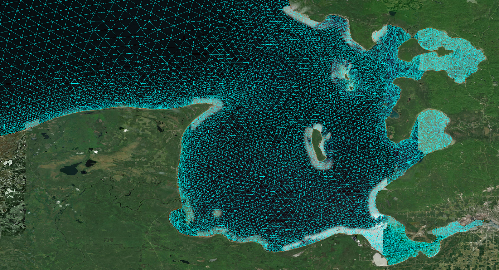
The primary goal of the SHARC project is to track and analyze HABs in Saginaw Bay in near-real-time. Saginaw Bay is a shallow, bloom-prone embayment where wind and currents can quickly shift the location of toxic algae. While GLERL has monitored these waters since 2010, the SHARC project will track harmful algal blooms as they occur this summer.

The “brain” of this mission is MBARI’s third-generation environmental sample processor (3G ESP). Integrated directly into the surface vessel, the 3G ESP automatically collects water samples and uses Surface Plasmon Resonance (SPR) to analyze them for toxins such as microcystins while still out on the water. It also preserves samples for later “omics” analysis, giving us a molecular-level look at the algal community and its genetic potential for toxicity that can affect drinking water quality. The SHARC system allows us to provide timely, actionable data to water managers and the public.

During the mission, SHARC will serve as a flexible, event-response platform. If a heat wave, passing weather front, strong winds, satellite imagery, or reports from people on the water suggest a bloom may be forming or moving to a new area, scientists can send SHARC to areas of concern to test the water directly. By pairing real-time toxin measurements with samples saved for later laboratory analysis, SHARC will help identify where blooms are occurring, how toxic they are, and what is causing them. and how they are changing over time. These observations will help scientists better understand HABs in Saginaw Bay and support informed decision-making for those who rely on its waters.

Images from the Sky

The SeaTrac ASV is not the only technology at use in the SHARC project. To find the best sampling spots, we’re using an Uncrewed Aerial System (UAS)—a hexacopter drone equipped with a specialized hyperspectral imager. The hyperspectral camera detects the unique light signature of cyanobacteria, identifying “hotspots” of high HAB biomass. Flying at altitudes below 400 feet, the imager provides high-resolution “eyes in the sky” that can see below the clouds that often block satellite views. The imagery also fills in the gaps nearshore, where shallow waters can disrupt satellite data due to low image resolution or light reflections from the lake floor. Scientists then use this data to help direct the ASV to the hot spots to determine if they contain the harmful algal bloom toxin.

While the hyperspectral data can identify the presence and extent of a bloom, it can not determine toxin levels. The water must then be sampled in order to determine the toxin level, and that is when the SeaTrac ASV moves in.

Setting Sail this July

Deployment of the SeaTrac ASV will operate out of Sebewaing, MI, with the craft conducting both underway sampling and holding location near a target station in locations as far northeast as Caseville, MI. 

As we set sail this July, we’re looking forward to the insights this mission will bring to help monitor local water quality, keep boaters and beachgoers safe from toxins, and protect our beloved Great Lakes. If you’re out on Saginaw Bay this summer and spot the SeaTrac vessel in action, be sure to snap a photo from a safe distance of 200 feet or more and share it with us! We love seeing our research through the eyes of the community. Tag your posts with #freshwaterSHARC to join the conversation as we work to keep our waters safe for everyone.

It was a cold and icy winter in 2025-2026. Lake ice affects everything from snowfall and fishery populations to recreational activities and the multibillion-dollar commercial shipping industry, making Great Lakes ice cover data highly valuable. However, once winter arrives boats and buoys are removed from the water to protect them from ice, so the NOAA Great Lakes Environmental Research Laboratory (GLERL) monitors the Great Lakes by taking to the sky. GLERL has been using a technique called hyperspectral imagery for over a decade to monitor Great Lakes harmful algal blooms in the summer. This method, which uses cameras to collect wide band data from across the electromagnetic spectrum, can also be utilized to monitor lake ice.

One possible method is monitoring ice conditions from the sky, using a camera that collects a wide band of data from across the electromagnetic spectrum. By using a technique called hyperspectral imagery, GLERL has been collecting data over the Great Lakes for over a decade, frequently to monitor harmful algal blooms during the summer. Starting in 2024, our researchers began to explore flying a hyperspectral camera to monitor lake ice during the winter.

What is hyperspectral data?

Hyperspectral data or imagery contains much more information than a visible image. Traditional images capture what a human eye sees (visible light spectra), which consists of three bands: red, green and blue. The ‘hyper’ in hyperspectral means that the data collected captures parts of light beyond what our eyes can see, such as the near-infrared (thermal/heat range). Instead of three bands like our eyes or a traditional camera captures, hyperspectral cameras capture over 150 bands. How does all that extra information fit into an image? Hyperspectral data isn’t analyzed as a flat 2D image, but forms a 3D data cube. Different materials reflect and absorb light in a unique way, creating a spectral fingerprint similar to the uniqueness of a human fingerprint. By collecting hyperspectral data we are able to shift from looking at an object to identifying it by its spectral fingerprint. A spectral signature plot (or spectra plot) provides a graphical representation of a selected pixel in a hyperspectral image. The x-axis represents the wavelength in nanometers while the y-axis represents the intensity, also referred to as brightness, which is a measure of the amount of light being reflected at a particular wavelength. The blue, green and red vertical lines indicate the specific bands used to render the current hyperspectral image; in Figure 2, which shows different hyperspectral images, they were selected to mimic the standard red-green-blue spectrum seen with a human eye.

The first step in hyperspectral data collection begins with outfitting a small aircraft – a Cessna 210 in our case – with the hyperspectral camera (Figure 3). Once the camera is installed, the pilot flies a pre-defined flight path surveying an area of interest. Throughout our most recent ice flight mission, the aircraft maintained a survey altitude of 10,500 ft, capturing high resolution ice data.

Quick Shifts, Complex Conditions

The Great Lakes are known for their propensity to change rapidly. Many know the phrase “if you don’t like the weather, wait five minutes”, and the lakes are no different. Figure 5 below shows three visible webcam images from the same viewpoint highlighting the shift of Lake Erie ice sheets across a three hour timeframe. Winds and currents have a dramatic impact on how quickly the ice moves. This shows how monitoring, prediction, and reporting ice conditions can be challenging.

How is Great Lakes ice tracked and forecast now? A combination of numerical models and satellites that use radar, visible and infrared imagery determine ice conditions. Ice condition information is crucial for shipping in the Great Lakes, as commercial shipping traffic still transects the lakes throughout the winter months when conditions allow – even when ice is present. However, existing methods to monitor and track ice in the Great Lakes have limitations: satellites only provide periodic static images, and numerical models require high-fidelity data for validation. To address these gaps, GLERL is exploring hyperspectral imaging as a way to improve current monitoring systems and improve model predictions.

After hyperspectral data is collected it can be processed multiple ways. One of the products from these ice flights is true color imagery. Figure 4 below consists of four north-to-south passes over Lake Erie when covered with ice. At first glance one can observe a few different features by eye in the visible imagery: wind-blown snow, rough ice, possibly open water and a wispy cloud that created a slight shadow.

Looking Forward

In addition to using airplanes, we can also use aerial drones to capture hyperspectral data. To leverage this emerging technology, GLERL established an aerial drone program in 2024. This provides a significantly different perspective since aerial drones fly much lower to the ground,  allowing them to capture much higher resolution images. Additionally, some drones are able to hover in one place while collecting data.

Collecting hyperspectral data from planes and drones is critical to understanding ice cover and ecology in the Great Lakes. By monitoring harmful algal blooms with hyperspectral imagery, we can safeguard drinking water intakes for millions of people, while also gaining insight into the dynamics of ecosystems in the lakes. Capturing hyperspectral ice cover data is fairly new but the potential payoff is big. Providing timely ice cover data at a resolution and accuracy never before available benefits all those that depend on the Great Lakes. Ice impacts everything from wildlife populations and health to the freighters that navigate the ice moving almost 200 million tons of materials each year, keeping our regional economy strong.

The ice features identified in Figure 4 are just the beginning of ice analysis based on hyperspectral data. More detailed analysis can confirm the ice classification (for example, determining different types or ice formation or thickness of ice) with more confidence and accuracy, thanks to the wealth of data that is embedded in a hyperspectral image. Advanced techniques are able to turn big datasets – including hyperspectral data – into valuable information. One technique is called deep learning, which allows an algorithm to study a big data set and then make predictions about that data. In our case, a deep learning algorithm  studied 150 bands of an image and then described more about the ice types than we would be able to tell by looking at it with our red-green-blue detecting eyes. This takes trial and error and requires us to have the “ground truth” in order to train and check the algorithm. Finally, GLERL also conducts an analysis of how Great Lakes ice conditions progressed throughout the previous winter. Comparing the past winter’s conditions to historical trends, helps us understand the key factors that influence ice formation, how ice conditions have changed over time, and how we might predict future ice cover. With an increase in both the quality and quantity of ice condition data, GLERL predictions will continue to improve services for a broad range of Great Lakes stakeholders.