Biological and Taxonomic Terms

Most of the terms in this section are used in the Species List Generator (https://www.glerl.noaa.gov/glansis/nisListGen.php). This search engine searches individual report data and returns a list of all species that have at least one report that fits the selected criteria, even if that report is not representative of the species' presence in the Great Lakes overall. For example, if you select a certain pathway from the 'Pathway' field, a species is included in the resulting list if any report assigned it to that pathway, which does not necessarily indicate that this is the primary pathway by which the species reached the Great Lakes (it may have been speculated for a single report, it may be a potential alternative pathway, or it may be indicating a pathway for spread within the Great Lakes). CAUTION: If any subselector is turned on here, when a user 'clicks through' the profile to the data table, the table includes ONLY specimens meeting the selection criteria. For example, if some reports of zebra mussels indicated their pathway as 'shipping ballast water' and others as 'unknown', then if you select 'shipping' as the pathway you will see only the data for points designated as 'shipping', not all the zebra mussel data. We highly recommend only using the pathway selector to generate the list, then resetting this search to 'all' before clicking through when a user actually wants to access all the data for a species on a particular pathway-related list. 

• Category (Species List Generator and results) – This feature of the Species List Generator searches based on whether or not the species is native to any portion of the selected geographic area.
• Nonindigenous – The species included in the GLANSIS nonindigenous list are those which are considered nonindigenous within the Great Lakes basin by meeting at least three of the following criteria (based on Ricciardi 2006):
1. the species appeared suddenly and had not been recorded in the basin previously;
2. it subsequently spreads within the basin;
3. its distribution in the basin is restricted compared with native species;
4. its global distribution is anomalously disjunct (meaning it contains widely scattered and isolated populations);
5. its global distribution is associated with human vectors of dispersal;
6. the basin is isolated from regions possessing the most genetically and morphologically similar species.
• Range Expander – The species included in GLANSIS on the 'range expander' list are those which are considered nonindigenous to a portion of the Great Lakes basin according to the above nonindigenous criterion but which have been identified in the peer-reviewed literature and/or by consensus of expert review to be native or cryptogenic in some portion of the basin. Cryptogenic species are those species that cannot be verified as either native or introduced (after Carlton, 1996). These include species that may have been identified as invasive by one researcher, but for which a literature review reveals conflicting opinions. The range expander list includes cryptogenic species when the population is clearly nonindigenous to a portion of the basin or if the population is suddenly expanding (such as formerly rare species becoming dominant), or changing growth forms, indicating the possibility a that non-native strain is invading (such as solitary species becoming colonial).


• Watchlist – The watchlist is intended to strike a balance between being precautionary and practical for support of early detection efforts. As of 2020, only those species assessed as likely to be introduced AND to be able to overwinter and reproduce in the Great Lakes are included in the watchlist. All species that have been assessed by our protocols (both those meeting the criteria for the watchlist below and those not) are included in the Risk Clearinghouse portion of the data (https://www.glerl.noaa.gov/glansis/riskAssessment.html).  
• Geographic criterion – Lives in a known donor region (such as rivers adjacent to Great Lakes, inland lakes in the Great Lakes region, western Europe, the Ponto-Caspian region) or in a zone with high specialization, species pool, or climate conditions that match the Great Lakes.
• Aquatic criterion – The criterion of including only aquatic species is unchanged. USDA wetland indicator status is used as a guideline for determining whether wetland plants should be included in the list: OBL, FACW, and FAC wetland plants are included in this list as aquatic; FACU and UPL plants are not. Waterfowl, amphibians, reptiles, and mammals are not currently included.
• Establishment criterion - Not already established in the Great Lakes, but assessed as 'likely' to become so in peer-reviewed literature or via our assessment (TM-169) as follows:
1. Vector Subcriterion – A transport vector currently exists that could move the species into the Great Lakes. The species is likely to tolerate/survive transport (including in resting stages) in the identified vector. The species has a probability of being introduced multiple times or in large numbers. And...
2. Reproduction and Overwintering Subcriterion – Based on known tolerances or climate matching, the species is likely to be able to successfully reproduce and overwinter in the Great Lakes. And...
3. Impact Subcriterion – The species has been known to impact other systems which it has invaded or is assessed as likely to impact the Great Lakes system.

OR

1. The species has been officially listed as a potential invasive species of concern by federal, state or provincial authorities with jurisdiction in the Great Lakes basin.

The original GLANSIS Watchlist of 67 species primarily represented a synthesis of research conducted between 1998 and 2012. As a result, it may not fully reflect the effect which regulations established after that period have had or will have on vectors of introduction (such as ballast water, aquaculture, live food trade, bait). 

• Status (Species List Generator, species profiles)
• All – Setting the Status field to 'All' returns all data about the species that fit the selected criteria, regardless of status. The status of a species may be categorized as any of the following: 'Established, 'Reported,' 'Locally Established, 'Failed,' 'Stocked,' 'Extirpated,' 'Eradicated,' or 'Unknown.' Only the first two of these options ('Established' and 'Reported') are individually searchable.  


• Established – Reproducing and overwintering in any watershed of the Great Lakes. This term is used only in the Species List Generator; it is being phased out of the species profiles. Currently, GLANSIS' concept of establishment differs from that of Darwin Core, in which 'establishment' is viewed as a process defined by a series of 'degrees of establishment' rather than as a state. 


• Reported – Species was observed somewhere in the Great Lakes below the ordinary high water mark, but is not known to be established in the region. 


• Established or reported – When a species is categorized as 'established,' previous data points categorizing it as 'reported' are not removed from the database. This option returns only data in which species have been categorized as either 'established' or 'reported,' while excluding data points that use any of the other Status options. Selecting this option will usually result in the same species list as selecting the 'All' option (species must have at least one record as established in order to be listed as established), but it will not pull up data points that are not either 'established' or 'reported' - for instance, species that have records ONLY for 'failed', 'extirpated', 'stocked', etc. are excluded. If you click on the name of a species in the resulting list, then click the 'Full list of USGS occurrences' link in the species profile, the list of occurrences will only contain data about established or reported populations, not data about other status options. 
• Group (Species List Generator, Map Explorer, Species Level Risk Assessments Explorer) The Group terms are from the USGS Nonindigenous Aquatic Species controlled vocabulary. The chart below maps the USGS Group terms to the corresponding taxa from the Integrated Taxonomic Information System (ITIS). Note that the ‘Taxonomic Scope’ field in the Methods Explorer does not use the USGS controlled vocabulary.
  
  All of the following groups are searchable in the Species List Generator, but bacteria and viruses are currently excluded from the Map Explorer.

These additional groups are available only in the Risk Assessment Clearinghouse - Methods Explorer or Species Risk Explorer:

• Scientific Name (Species List Generator and results) – Name agreed to by taxonomists internationally. Usually the scientific name is given by the discoverer, but sometimes organisms are renamed based on new knowledge of their genetic relationships to other organisms. Properly, the scientific name includes the genus name and species name, both in italics, e.g., humans are Homo sapiens. The Integrated Taxonomic Information System (ITIS - itis.gov) is the primary authority consulted to resolve conflicting scientific names.


• Common Name (Species List Generator and results) – The non-scientific name by which a species is colloquially known most commonly in the US. The list generator 'common name' selector also searches the synonym field for alternative spellings and alternative common names.  


• Synonyms and other names (Species profiles) – Short list of synonyms (i.e., older/invalid scientific names) or alternate common names, including alternate spellings. In the case of an older/invalid scientific name, the source of that name will be listed. This field includes all common alternative spellings of species names (and is included in searches in the list generator), but is not exhaustive.


• Continent of Origin (Species List Generator results) – Indicates the species' native range. It does not necessarily mean the source of a species' introduction to the United States; a species could be introduced from another non-native location. For example, a species of fish native to Europe could be introduced to South America, and then from South America to Florida. In this case, the continent of origin would be Europe.
• Year first collected (Species List Generator results) – The year in which the species was first collected anywhere in the selected geography.


• Identification/description of species (Species profiles) – Description of physical and occasionally behavioral characteristics by which the species can be identified and distinguished from morphologically similar native species.


• Size (Species profiles) – Approximate size in SI units. This number is the standard length or total length for fishes, carapace length for crustaceans, shell width for bivalves, and alternate or comparable size measurements for other taxonomic groups.


• Native range (Species profiles) – Brief description of the species' native range.


• Ecology (Species profiles) – Basic ecology and biology, such as information on preferred habitat, diet, fecundity, breeding/spawning season, etc.


• Pathway (Species List Generator)

The following terms are options for the Pathway field in the Species List Generator:

• Aquaculture – Fish, shrimp, or other deliberately cultured aquatic organisms that have escaped from aquaculture facilities.
• Canals – Species successfully navigated a man-made canal to a new drainage. Example: sea lamprey (Petromyzon marinus) entered Lake Erie and the upper Great Lakes through the Erie Canal.
• Dispersed – Species not deliberately/accidentally moved (i.e., unrelated to human interaction) from one area to another.
• Dispersed flood – Species move across waterbodies due to flooding/high water.
• Dispersed current – Species move from one region to another due to drift/transport on currents (e.g., South American swimming crab Callinectes bocourti on Atlantic coast of Florida).
• Dispersed wind – Species move from one region to another due to aeolian transport (e.g., wind-dispersed seeds of emergent vegetation such as cattails)
• Escaped captivity – General category for all species that escape from captivity; indicates accidental as opposed to intentional/deliberate release. Only used when the pathway cannot be identified as one of the more specific subcategories.

The generic 'Escaped captivity' category cannot be used as a search term in the Species List Generator. The following subcategory can be used as a search term:

• Pet escape – Non-aquarium pets (e.g., snakes, turtles) that were not deliberately released. This category has been phased out in favor of 'Released pet' but older data still uses the 'Pet escape' category.

The remaining subcategories can only be accessed by selecting 'All' in the Species List Generator:

• Escaped captivity aquaculture
• Escaped captivity farm
• Escaped captivity fur farm
• Escaped captivity pond
• Escaped captivity research
• Escaped captivity zoo
• Pet escape – Non-aquarium pets (e.g., snakes, turtles) that were not deliberately released.
• Planted – Plant species intentionally placed into a water body; used to indicate a sanctioned event by an authorized party.
• Planted erosioncontrol – Introduced to mitigate/reduce erosion.
• Planted food – Introduced for human consumption.
• Planted forage – Introduced for non-human consumption.
• Planted ornamental – Planted as an ornamental, typically in landscaping. Not intended to be directly released into the wild, but 'escaped' the original setting.
• Planted restoration/mitigation – Introduced for habitat restoration.
• Planted wildlife habitat – Planted for wildlife habitat in wild or semi-wild areas. 
• Released – General category for all released species; indicates intentional as opposed to accidental (escape) release, and non-sanctioned as opposed to sanctioned (stocked) release. Only used when the pathway cannot be identified as one of the more specific subcategories. 

The generic 'Released' category cannot be used as a search term in the Species List Generator. The following two subcategories can be used as search terms:

• Aquarium release – Aquarium species that are let go (e.g., fish, plants, snails); typically unauthorized deliberate release.
• Baitrelease – Species released by anglers after use as bait (e.g., minnows, crayfish, salamanders). 

The remaining subcategories can only be accessed by selecting 'All' in the Species List Generator:

• Released for food
• Released lab animals
• Released pet
• Shipping – Generic pathway term for any species transported via large commercial ship unless the introduction is specifically known to have occurred due to ballast water, hull fouling, or solid ballast. Species transported by smaller, personal watercraft are classified under 'hitch hiker on small watercraft.'
• Shipping ballast water – Species transported in ballast water of commercial shipping vessels (e.g., zebra mussels, introduced plankton in the Great Lakes).
• Shipping hull fouling – Species that attach to hulls of ships (e.g., tunicates, bryozoans, and mussels). Most fouling species also have larval stages that can be transported by ballast water. 
• Shipping solid ballast – Species transported in/on solid ballast or soil. Generally used for historic introductions; solid ballast not used in shipping for many decades. Usually limited to plants/algae.
• Stocked – Animal species intentionally placed in large numbers in a water body; used to indicate a sanctioned event by an authorized agency. Non-sanctioned introductions by non-sanctioned parties are categorized under 'Released.'
• Stocked aquaculture – High density stocking of species used as human food source into small or enclosed areas.
• Stocked escaped – Species stocked into one waterbody and escaped into another waterbody. For example, rainbow smelt (Osmerus mordax) were stocked in a lake in northern Wisconsin, but escaped and moved into the Great Lakes.
• Stocked for biocontrol – Species stocked for control of another invasive species (e.g., grass carp, cane toad).
• Stocked for conservation – Endangered species moved to a new area to increase its chances of survival (e.g., various desert pupfish Cyprinodon spp.)
• Stocked for food – Stocked as a food source for humans (e.g., common carp).
• Stocked for forage – Generally small species (minnows, silversides) stocked as food for larger, predatory species (i.e., not for human consumption).
• Stocked for research – Species stocked for experimental purposes.
• Stocked for sport – Species stocked for sport fishing, usually large predatory fish (e.g., walleye, pike, bass, sunfish, salmon, trout).
• Stocked illegally – Species not stocked by the state, but by individuals without proper authority.
• Stocked misidentified – Agency stocked a species mistaken for another (e.g., green sunfish mistaken for bluegill sunfish).

The following categories can only be accessed by selecting 'All' in the Species List Generator:

• Hitch hiker – Species attached or concealed on another organism or object and unknowingly transported to another non-native location.

While the 'Hitch hiker' category as a whole can only be accessed by selecting 'All', one subcategory, 'Hitch hiker in aquaculture', is included in the 'Aquaculture' pathway. The other types of hitch hiker are as follows: 

• Hitch hiker on small watercraft
• Hitch hiker in aquaculture
• Hitch hiker on aquatic plants
• Hitch hiker on imported logs
• Hitch hiker on imported plants
• Hitch hiker on packing material
• Hitch hiker on plants
• Hitch hiker on oil platforms
• Hitch hiker with oysters
• Hitch hiker on scuba gear
• Hitch hiker with stocked fish
• Hitch hiker with tunicates
• Hitch hiker on waterfowl
• Hybridized – The hybrid was not introduced, but resulted from an introduced parent species breeding with a native species.
• Unknown –  Reports not assigned to a particular vector.
• Means of Introduction (Profile) – Explanation of how the species was introduced to the U.S.  Often includes more detailed and/or speculative information about the original pathway for the species introduction.  Means of introduction in the profile is written for the species level, not the individual report.

Ecological Terms

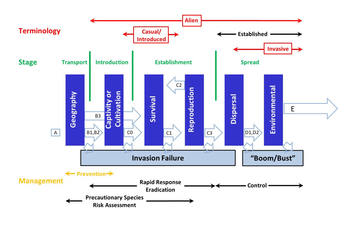
Figure 1: Proposed framework by Kocovsky et al. (2018; Figure 1), modified from Blackburn et al. (2011; Figure 1), for management alternatives for non-native and invasive species. Approximate color schemes from Blackburn et al. are retained with changes by Kocovsky et al. in black text.

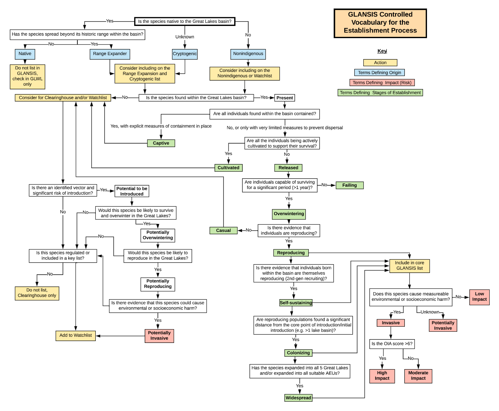
Figure 2: GLANSIS controlled vocabulary for the establishment process. The Methods Explorer searches literature by a variety of authors, who may either use different terminology to describe the establishment process than GLANSIS or use different definitions for the same terminology that GLANSIS uses.

Considerations (Methods Explorer and results, Species Level Risk Assessments Explorer results) – The GLANSIS Risk Clearinghouse Methods Explorer enables searching for Risk Assessments Method Literature by features of the methods. Searchable features include whether the method addresses each of the following considerations. The Species Level Risk Assessments Explorer enables searching for risk assessment literature by taxonomic group. The results of this search engine indicate whether the literature addresses each of the following considerations. 

• Arrival –The initial stage of the establishment process during which the non-native species initially enters the system of interest. Represented in Figure 1 by the elements to the left of C0.
• Both Transport and Introduction phases (per figure 1) are considered as parts of Arrival for the purposes of the Risk Assessment Clearinghouse Method Explorer.  The Methods Explorer scores each method (Y/N) only on whether or not it considers any information about this phase of the establishment process.  Methods may differ substantially in the evidence used to draw conclusions about this phase.
• In the Species Level Risk Assessments Explorer, the term 'Introduction' is used in place of 'Arrival.' 
• The GLANSIS Risk Assessments (used for Watchlist species) use the term 'Introduction Potential' ['Potential to be Introduced' in the GLANSIS Vocabulary Flowchart] for the segment of the risk assessment which considers the Arrival phase. Evidence examined in this section focuses on the 6 common vectors of introduction to the Great Lakes: Dispersal, Hitchhiking, Unauthorized intentional release, Stocking/Planting & Escape from Recreational Culture, Escape from Commercial Culture, and Shipping, as follows:
• Does this species occur near waters (natural or artificial) connected to the Great Lakes basin* (e.g., streams, ponds, canals, or wetlands)? (*Great Lakes basin = below the ordinary high-water mark, including connecting channels, wetlands, and waters ordinarily attached to the Lakes)
• What is the proximity of this species to the Great Lakes basin?
• Is this species likely to attach to or be otherwise transported by, or along with, recreational gear, boats, trailers, fauna (e.g., waterfowl, fish, insects), flora (e.g., aquatic plants), or other objects (e.g., packing materials), including as parasites or pathogens, entering the Great Lakes basin?
• What is the proximity of this species to the Great Lakes basin?
• Is this species sold at aquarium/pet/garden stores ('brick & mortar' or online), catalogs, biological supply companies, or live markets (e.g., purchased for human consumption, bait, ornamental, ethical, educational, or cultural reasons) and as a result may be released into the Great Lakes basin?
• How easily is this species obtained within the Great Lakes region (states/provinces)?
• Is this species being stocked/planted to natural waters or outdoor water gardens around the Great Lakes region?
• What is the nature and proximity of this activity to the Great Lakes basin?
• Is this species known to be commercially cultured in or transported through the Great Lakes region?
• What is the nature and proximity of this activity to the Great Lakes basin?
•  Is this species capable of surviving adverse environments (i.e. extreme temperatures, absence of light, low oxygen levels) and partial-to-complete ballast water exchange/BWE (e.g., is euryhaline, buries in sediment, produces resistant resting stages, has other attributes or behaviors facilitating survival under these conditions)?
• Does this species occur in waters from which shipping traffic to the Great Lakes originates?
• Survival– The stage marked as 'Survival' in Figure 1. 
• Establishment – The stage at which a species is reproducing and overwintering. Represented by the section of Figure 1 between C0 and C3. Since survival is an element of establishment, a method that considers survival is always categorized as considering establishment as well. 

Each method included in the Risk Clearinghouse may have subtly different definitions and criteria and the original source should always be consulted for an exact definition and full understanding of this term.

The GLANSIS Risk Assessment method includes survival and spread as subsets of establishment, with the detailed criteria as follows:

• Invasive Biological/Ecological Attributes
• How would the physiological tolerance of this species (survival in varying temperature, salinity, oxygen, and nutrient levels) be described?
• How likely is it that any life stage of this species can overwinter in the Great Lakes (survive extremely low levels of oxygen, light, and temperature)?
• If this species is a heterotroph, how would the flexibility of its diet be described?
• How likely is this species to outcompete species in the Great Lakes for available resources?
• How would the fecundity of this species be described relative to other species in the same taxonomic Class?
• How likely are this species' reproductive strategy and habits to aid establishment in new environments, particularly the Great Lakes (e.g., parthenogenesis/self-crossing, self-fertility, vegetative fragmentation)?
• Environmental Compatibility 
• How similar are the climatic conditions (e.g., air temperature, precipitation, seasonality) in the native and introduced ranges of this species to those in the Great Lakes region?
• How similar are other abiotic factors that are relevant to the establishment success of this species (e.g., pollution, water temperature, salinity, pH, nutrient levels, currents) in the native and introduced ranges to those in the Great Lakes?
• How abundant are habitats suitable for the survival, development, and reproduction of this species in the Great Lakes area (e.g., those with adequate depth, substrate, light, temperature, oxygen)?
• How likely is this species to adapt to or to benefit from the predicted effects of climate change on the Great Lakes freshwater ecosystems (e.g., warmer water temperatures, shorter duration of ice cover, altered streamflow patterns, increased salinization)?
• How likely is this species to find an appropriate food source (prey or vegetation in the case of predators and herbivores, or sufficient light or nutrients in the case of autotrophs)?
• Does this species require another species for critical stages in its life cycle such as growth (e.g., root symbionts), reproduction (e.g., pollinators, egg incubators), spread (e.g., seed dispersers), or transmission (e.g., vectors)?
• How likely is the establishment of this species to be aided by the establishment and spread of another species already in the Great Lakes?
• How likely is establishment of this species to be prevented by the herbivory, predation, or parasitism of a natural enemy that is already present in the Great Lakes and may preferentially target this species?
• Propagule Pressure
• On average, how large and frequent are inoculations (introduction events) from the potential vectors identified in Section A for this species? (What is the total number of individuals introduced?)
• History of Invasion and Spread
• How extensively has this species established reproducing populations in areas outside its native range as a direct or indirect result of human activities?
• How rapidly has this species spread by natural means or by human activities once introduced to other locations?
• Are there any existing control measures in the Great Lakes set to prevent the establishment and/or spread of this species?

• Spread – The section of Figure 1 between C3 and D2.
• Ecological Impacts – See Impact Terms section of dictionary.
• Socioeconomic Impacts – See Impact Terms section of dictionary. 
• Manageability –An assessment considers manageability if it contains any statements about whether a species can be managed and/or how easy or difficult management is for that species.

NOAA GLANSIS watchlist method: https://www.glerl.noaa.gov/pubs/tech_reports/glerl-169/tm-169.pdf  

Management (Species profiles) – Management efforts related to controlling or eradicating species.

• Regulations – Legislation or agency policies aimed at managing species.
• Control – Management by way of intervening in the ecosystem. There are three kinds of control:
• Biological – The release of one species, usually a predator, to control the population of another species. 
• Physical – Physicalinterventions in the environment, such as dredging a body of water or constructing a barrier.
• Chemical – The use of a chemical such as a pesticide or herbicide that kills the organism. 

Geological and Environmental Terms

• Lake (HUC) (Species List Generator, Map Explorer, species profiles) - All GLANSIS records are point data, but each point is assigned the corresponding Hydrologic Unit Code (HUC). This selector in the Species List Generator searches for individual records based on HUCs. Species are included only if a record is found for the HUC. An explanation of HUCs can be found at https://water.usgs.gov/GIS/huc.html.  The Map Explorer contains a HUC data layer from https://hydro.nationalmap.gov/arcgis/rest/services/wbd/MapServer.
• Basemap (Map Explorer)

The following layers are from ArcGIS by way of the Great Lakes Aquatic Habitat Framework.

• Topographic – The map includes administrative boundaries, cities, water features, physiographic features, parks, landmarks, highways, roads, railways, and airports overlaid on land cover and shaded relief imagery for added context. This basemap was compiled from a variety of best available sources from several data providers, including the U.S. Geological Survey (USGS), U.S. Environmental Protection Agency (EPA), U.S. National Park Service (NPS), Food and Agriculture Organization of the United Nations (FAO), Department of Natural Resources Canada (NRCAN), GeoBase, Agriculture and Agri-Food Canada, Garmin, HERE, Esri, OpenStreetMap contributors, and the GIS User Community.


• National geographic – This map was developed by National Geographic and Esri and reflects the distinctive National Geographic cartographic style in a multi-scale reference map of the world. The map was authored using data from a variety of leading data providers, including Garmin, HERE, UNEP-WCMC, NASA, ESA, USGS, and others. This reference map includes administrative boundaries, cities, protected areas, highways, roads, railways, water features, buildings and landmarks, overlaid on shaded relief and land cover imagery for added context. 


• Oceans – This map features marine bathymetry, as well as marine water body names, undersea feature names, and derived depth values in meters. Land features include inland waters and roads overlaid on land cover and shaded relief imagery. The map was compiled from a variety of best available sources from several data providers, including General Bathymetric Chart of the Oceans GEBCO_08 Grid, National Oceanic and Atmospheric Administration (NOAA), and National Geographic, Garmin, HERE, Geonames.org, and Esri, and various other contributors. The map was designed and developed by Esri. 


• Gray – This map draws attention to thematic content by providing a neutral light gray background with minimal colors, labels, and features. Only key information is represented to provide geographic context, allowing the data and patterns to come to the foreground. This map was developed by Esri using HERE data, Garmin basemap layers, OpenStreetMap contributors, Esri basemap data, and select data from the GIS user community.


• Dark gray – This map draws attention to thematic content by providing a neutral dark gray background with minimal colors, labels, and features. Only key information is represented to provide geographic context, allowing the data and patterns to come to the foreground. This map was developed by Esri using HERE data, Garmin basemap layers, OpenStreetMap contributors, Esri basemap data, and select data from the GIS user community. 


• Imagery – World Imagery provides one meter or better satellite and aerial imagery in many parts of the world and lower resolution satellite imagery worldwide. The map features Maxar imagery at 0.5m resolution across the United States. In addition to commercial sources, the World Imagery map features high-resolution aerial photography contributed by the GIS User Community. 


• Shaded relief – This map portrays surface elevation as shaded relief. The shaded relief imagery was developed by Esri using GTOPO30, Shuttle Radar Topography Mission (SRTM), and National Elevation Data (NED) data from the USGS.


• USA topographic – This map presents land cover imagery for the world and detailed topographic maps for the United States. The map includes the National Park Service (NPS) Natural Earth physical map at 1.24km per pixel for the world at small scales, i-cubed eTOPO 1:250,000-scale maps for the contiguous United States at medium scales, and National Geographic TOPO! 1:100,000 and 1:24,000-scale maps (1:250,000 and 1:63,000 in Alaska) for the United States at large scales. The TOPO! maps are seamless, scanned images of United States Geological Survey (USGS) paper topographic maps.

• Surface Layers (Map Explorer)
• General 

The following layers are compiled by and separately available from the Great Lakes Aquatic Habitat Framework (https://www.glahf.org/).

• Geomorphology depth – This layer color-codes the map of the lakes according to the depth of the water. Depth in meters is represented as a continuous variable, with darker shades of blue representing greater depths. The bathymetry for the Great Lakes was obtained from NOAA National Centers for Environmental Information.  


• Geomorphology substrate – Thislayer assigns a different color to each substrate, or type of sediment underlying the waters of the lakes: clay, mud, sand, hard, and unknown. Substrate for the bottom of the Great Lakes in the offshore regions was digitized from peer reviewed publications.  In the coastal and nearshore zones, the shoreline material descriptions of the U.S. Army Corps of Engineers (USACEs; 2012) were extended to 30 m of depth and confirmed by researchers across the Great Lakes and benthic sampling data. In Lake Erie, the Lake Erie Habitat Task Group has collected fine scale substrate data from tow, grab sample, and underwater video data to support management decisions for fish habitat.  Several other locations included fine scale substrate data such as the Illinois waters of Lake Michigan, and in the nearshore areas of Minnesota, Lake Superior.


• Spring surface temperatures – Averaged spring estimates of surface water temperature were calculated from remote sensing estimated daily data (NOAA Great Lakes CoastWatch) from 1995 to 2013. This layer shows the average spring surface temperature from 2006-2012. Spring is defined as April 1 to May 31, and temperatures are binned in increments of 2º C.


• Summer surface temperatures – See Spring surface temperatures (previous bullet point). This layer shows the average summer surface temperature from 2006-2012. Summer is defined as July 1 to August 31, and temperatures are binned in increments of 2º C.


• Cumulative degree days – Cumulative degree-days are an index of the thermal energy experienced by organisms over a given period of time (Venturelli et al. 2010). CDD was calculated as the sum of mean daily epilimnetic water temperatures during ice free days (above a base of 0°C) from January 1 through December 31 and averaged from 2006 to 2012 to capture a range of variation in annual temperatures. In the nearshore and offshore zones (> 5 m), modeled vertical water temperature was used to calculate a mean daily temperature for the depth range of 0-20 m, representing average epilimnetic temperatures (http://www.glerl.noaa.gov/res/glcfs/). In shallow nearshore zones (< 5 m), where modeled temperatures are relatively coarse grained, mean average water temperature was calculated from surface water satellite estimates (http://coastwatch.glerl.noaa.gov/). The resultant CDD estimates from the shallow nearshore, the deep nearshore, and offshore zones were combined into a composite data layer. This layer represents CDD as a continuous variable without breakpoints. The 'Thermal Regime' layer listed under the heading 'Ecological Classification' below also maps CDD, but uses sharp breakpoints corresponding to fish guild preferences.


• Ice duration – Since 1973 ice cover has been interpolated from remotely sensed images.  The daily percent ice cover (concentration) is available from 1973-2002 from the NOAA Great Lakes Ice Atlas, and since 2002 the NOAA Great Lakes Environmental Research Laboratory has continued to make observed days of ice available. GLAHF summarized the data into monthly and annual ice cover concentration and an annual ice duration index (in days) for the years 1973-2013.


• Upwelling – Upwellings occur when strong surface winds push warm surface water away from the coastline, which is replaced by cold, nutrient rich water that wells up from deeper areas below. Upwellings were mapped from NOAA's Great Lakes CoastWatch Node Great Lakes Surface Environmental Analysis product following methods from Plattner et al. (2006). The data shown here averages the number of days per year on which upwelling occurred between 2006 and 2012. Upwelling frequency is represented as a continuous variable, with darker shades of purple representing a greater frequency.
• Ecological Classification 

The following layers are from the Great Lakes Aquatic Habitat Framework.

• Aquatic ecological units – An ecological classification with 77 types, each of which depicts a unique combination of depth, thermal regime, mechanical (or hydraulic) energy, and tributary influence (Riseng et al. 2018). GLANSIS Map Explorer contains a layer for each of these factors, all of which are imported from GLAHF (https://www.glahf.org/classification/).  The chart to the right depicts the ecosystem-based mapping of aquatic ecological units of the Great Lakes. Four variables (depth, cumulative degree-days, mechanical energy, and tributary influence) were combined hierarchically across three ecological zones (coastal margin, nearshore, and offshore) as shown in the chart below: depth, cumulative degree-days, mechanical energy (i.e., relative exposure index and currents), and tributary influence. Each variable was characterized by three or four criteria that defined ecological breaks in key drivers. Each possible aquatic ecological unit (AEU) type is shown by a unique color. The cells that contain diagonal black lines on a white background represent AEU types that do not exist in the Great Lakes. 
• Depth – The aquatic ecological classification identifies five bathymetric thresholds that were related to littoral energy, aquatic vegetation extent, stratification limits, and light extinction. The extent of the nearshore zone was defined as < 30 m depth contour in all Great Lakes, except Lake Erie where the extent was defined as the greater of a 15 m depth contour or 5 km from shore to capture the well-mixed zone. A zone unique to Lake Erie, the shallow offshore, was defined as occurring between 15 m and 30 m due to a difference in currents and variation in the extent and depth of annual summer stratification (Rucinski et al. 2010). In the offshore (> 30 m depth) two zones were defined: deep and profundal. The deep offshore zone was defined as the region from 30—100 m in depth. The 100-m depth represents 1% limit of light penetration (Wetzel 2001) and where the photosynthesis to respiration ratio is < 1. Depths greater than 100 m were classified as the profundal offshore zone. GLAHF obtained bathymetric data from the National Oceanic and Atmospheric Administration (NOAA) National Centers for Environmental Information (NCEI). The original raster in 3-second resolution (approximately 90 m) was standardized to the GLAHF framework grid and anomalous depth values incongruous with depth data from the NOAA Nautical Chart 14968 were removed. The 0-m depth was defined using the jurisdictional Ordinary High Water Mark (U.S. ACOE 1985), which was integrated with the high resolution shoreline including island polygons greater than 10 ha (Forsyth et al. 2016) and enforced as the land-water boundary.
  
  
• Thermal regime – Thermal regime is the spatial and temporal variability in water temperature measured in terms of cumulative degree days (CDD). For an explanation of CDD, see the 'Cumulative degree days' bullet point under the 'General' heading. CDD was here classified into low, moderate, and high categories based on fish guild preferences (Wehrly et al. 2012a and Bailey et al. 2004), which correspond to the thermal habitat requirement of warmwater (high), coolwater (moderate), and coldwater (low) fish guilds. The layer uses a threshold of 3,900 degree days to delimit the break between medium and high categories and 3,000 degree days to delimit the break between medium and low categories. The 'Cumulative Degree Days' layer listed under the heading 'General' above also maps CDD, but maps it as a continuous variable without breakpoints.


• Mechanical energy – Mechanical energy mainly represents the energy transferred from wind to water resulting in waves, longshore currents, gyres, seiches, and upwelling. The mechanical energy layer uses two variables to represent mechanical energy associated with coastal and offshore water motion: a relative exposure index for the coastal margin and shallow nearshore zones (< 5 m) that summarized wave energy; and a generalization of circulation patterns for deep nearshore and deep and profundal offshore areas. The relative exposure index (REI) is a wind speed, direction, and frequency weighted measure of effective fetch (Keddy 1982). Using the methods and ArcGIS tool developed by Rohweder et al. (2012), REI was calculated for each lake applying the wind data summaries for the nearest buoy to a given area of lake, which were then combined into a Great Lakes wide REI map for coastal margin and shallow nearshore zones. REI was classified into low, moderate, and high using natural breaks.

For deep nearshore and deep to profundal offshore zones, GLAHF summarized published Great Lakes circulation patterns to map general patterns of surface water motion (Sheng and Rao 2006; Prakash et al. 2007; Schwab et al. 2009; Bennington et al. 2010; Beletsky et al. 2013). The directional (alongshore) current was defined as occurring from the 5-m isobaths to either the 30-m isobaths (15 m in Lake Erie) or 5 km from the high resolution shoreline, whichever distance was greater based on a compilation of studies and information describing circulation patterns (Beletsky et al. 1999; Rao and Schwab 2007; Kelly et al. 2015; and C. Troy (Purdue University, pers. comm. 2015)). The large-scale cyclonic/anti-cyclonic and mixed circulation patterns were mapped from the directional current boundary across the offshore zone using heads-up digitizing. 


• Tributary influence – The tributary influence variable represents the potential influence of tributary and coastal watersheds on coastal and nearshore zones. This variable was computed by first calculating the contributing watershed area of each tributary or coastal segment. Three classes of the tributary influence variable were used, based on tributary catchment area (Minns and Wichert 2005; Allan et al. 2013): low (< 30 km2, mean size of first and second order tributaries); moderate (30- 250 km2 , representing third and some fourth order tributaries), and high (> 250 km2 , representing ≥ fourth order tributaries). This variable is developed for the nearshore zones only, and offshore zones were assigned a value of '0'.
  
  The relative tributary size was then propagated into the lake based on a mathematical distance decay function weighted by depth. The decay equation assumed 10% of the initial flow value persisted at 15 km from the river mouth and 1% at 30 km distance (Allan et al. 2013), but was modified to weight distance by depth to allow the load to move more easily through shallow waters (< 5 m) and become entrained in the nearshore zone (Makarewicz et al. 2012). For the tributaries, the distance was calculated from the pour-point of each river mouth; for the coastal segments without tributaries, the distance was from the midpoint of the entire interfluve shoreline. To capture the flow of the connecting channels, an estimated watershed area was assigned based on the proportion of major contributing watersheds for each connecting channel (St. Marys, North Channel, St. Clair, Detroit and Niagara Rivers). For St. Marys, Detroit and Niagara Rivers the influence of the contributing lake was captured by further scaling it to the mean flow.
• Habitat Suitability 

The options under this heading in the 'Surface Layers' field of the Map Explorer correspond to layers derived from Wittman et al. (2017) and Kramer et al. (2017).Each of these layers contains a map representing the suitability of the Great Lakes for a particular species. If the layer is labeled with only the name of the species, e.g., 'Hydrilla' or 'Golden Mussel', the resulting map shows the least restricted habitat suitability model for that species. If the layer is labeled with the name of the species and one or more restricting factors, the resulting map shows a habitat suitability model restricted by those factors. The following terms are used in the layers derived from Wittman et al. and Kramer et al.

• Niche Centrality – The ecological niche of a species is the set of environmental conditions within which the species can persist. Niche centrality measures the tendency of these environmental conditions to occur in a geographic area on a scale from 0 to 1. The higher the niche centrality, the more often the area has the correct environmental conditions for the species.


• Benthic temp – Wittman et al. (2017) and Kramer et al. (2017) both base their benthic temperature calculations on the hydrodynamic model created by the NOAA Great Lakes Coastal Forecasting System (GLCFS). In this model, each of the Great Lakes is divided into 20 (in the cases of Lakes Huron, Michigan, Ontario, and Superior) or 21 (in the case of Lake Erie) vertical layers. Benthic temperature is derived from the bottom layer. In the layers from Wittman et al., benthic temp is factored into the growing degree days calculation (see next bullet point), while in the layers from Kramer et al., benthic temp itself is used as a restricting factor for Golden Mussel and Snakehead.


• GDD – Growing Degree Days(GDD) are a measure of heat accumulation relative to the base temperature below which a given plant cannot grow. Wittman et al. (2017) use benthic GDD data to determine the suitability of each lake individually as a habitat for the submersed aquatic macrophyte Hydrilla using the formula GDD = Tavg − Tbase, when Tavg ≥ Tbase. Tavg is the mean benthic temperature in the lake and Tbaseis 8º C, the minimum development threshold below which Hydrilla cannot grow. Selecting the option 'Hydrilla restricted GDD' in the Surface Layers field of the Map Explorer returns a map in which GDD is factored into the niche centrality calculation for Hydrilla. Only regions in which GDD ≥ 500 are considered a suitable habitat in this model. 


• SAV and wetlands – To restrict their grass carp model, Wittman et al. used a combined data layer representative of submersed aquatic vegetation (SAV) and wetland regions of the Great Lakes, given that the species is likely to utilize these habitats directly as a food resource and refuge. Kramer et al. similarly used an SAV and wetlands layer to restrict their Northern snakehead (Channa argus) model. Both papers used the same SAV and wetlands data. 
  
  SAV data were produced and provided by the Michigan Tech Research Institute (Brooks et al., 2015; MTRI, 2012; Shuchman et al., 2013). The data have a 30 m resolution and represent the extent of SAV in the optically shallow areas of lakes Huron, Michigan, Erie, and Ontario. The data were generated using an MTRI-developed, depth-invariant algorithm applied to Landsat satellite data. The satellite data were collected during the vegetative growing season during various year ranges. Specifically, vegetative growing seasons were determined by temperature and years varied by lake; Lake Erie, May–September 2006–2011; Lake Huron, March–September 2007–2011; Lake Michigan, April–May 2008–2011; Lake Ontario, April–September 2008–2011. Some portions of these lakes could not be classified due to high turbidity (Shuchman et al., 2013). Wittman et al. note that SAV data did not exist or were not available for Southern Green Bay and Lake Superior and thus were excluded from the SAV restriction for grass carp, while Kramer et al. note that SAV data did not exist or were not available for Lake St. Clair and Lake Superior. Data for the remaining Great Lakes were combined using the 'Mosaic to New Raster' tool in ArcToolbox in ESRI ArcGIS Desktop Version 10.2 (ESRI, 2014) with a cell size of 30 m. Classes 1 (light submerged aquatic vegetation) and 7 (dense submerged aquatic vegetation) were utilized.


• Photic zone – The uppermost zone of a body of water, in which the light that penetrates the water is sufficient to enable plants and phytoplankton to perform photosynthesis. Wittman et al. restricted the Hydrilla model by depth of the euphotic zone, i.e., the depth where only 1% of the surface photosynthetic available radiation (PAR) remains, to represent the limitation of water transparency and the maximum depth of Hydrilla colonization within a lake (Canfield and Langeland, 1985).


• Shoreline Layers (Map Explorer) 

The following layers are from the Great Lakes Aquatic Habitat Framework.

• Classification – Shoreline classifications have been compiled from NOAA's Environmental Sensitivity Index, Environment Canada's Environment Sensitivity Atlas, and the U.S. Army Corps of Engineers (ACOE) shoreline descriptors. The ESA data ranges in dates from 1987 through the late 1990s, and the ACOE shoreline descriptions are from the 2012 oblique imagery interpretation. 


• Sinuosity – The shoreline sinuosity is the measure of the meandering of a segment of shoreline, where a high value (near 1) means almost straight and a low value (near 0) means highly meandering. Shoreline sinuosity was calculated using the shoreline delineation compiled for the Great Lakes Hydrography Dataset. The GLHD shoreline was divided into 1km segments and sinuosity was calculated by dividing the length of the shoreline segment by the straight line distance between the beginning and end point of the segment.

Scholarship and Research Terms

The terms in this section are used exclusively in the Risk Assessment Methods Explorer (https://www.glerl.noaa.gov/glansis/raExplorer.html).

• Publication Type (Methods Explorer) 
• Peer – Peer-reviewed literature appears in published scientific journal articles or books, is indexed by most scientific search engines (accessible to technical audiences) and generally have been subject to a third-party, (usually blind) peer-review process.
• Gray – Gray literature is information produced outside of traditional publishing and distribution channels, and can include reports, policy literature, theses and dissertations, working papers, newsletters, government documents, speeches, white papers, urban plans, and so on. Gray literature often is reviewed by the agency/institution, but not typically subject to a blind peer-review process. Gray literature is often difficult to access outside the specific institutional repository.
• Web – Web sources are taken from the internet, so they are readily accessible to the general public but not typically subject to a review process (though agency/institution review processes vary).
• Geographic scope (Methods Explorer and results) – This field selects the geographic range of the original methodology. For example, the geographic scope of NAS is the US, while the geographic scope of GLANSIS is the Great Lakes basin or the Great Lakes below the ordinary high water mark. Care should be taken in extrapolating results of methods conducted for other geographic scopes to the Great Lakes.


• Taxonomic scope (Methods Explorer and results) – This field selects the taxa for which the method was designed. Risk Assessments are often designed to be used with specific taxa and ask for data inputs that are specific to those particular taxa. For example, Notre Dame's STAIR method has separate assessments (i.e., different methods) for evaluating fish and mollusks.


• Assessment Type (Methods Explorer and results)
• Qualitative – Assessment based on non-numerical data. 
• Quantitative – Assessment based on numerical data.
• Scenario (vector) associated risk – Assessment in which multiple possible future scenarios are assessed for risk, with each risk assessment taking the same set of factors into account. 
• Semi-quantitative – Assessment in which qualitative data is collected, then assigned numerical values to permit quantitative analysis.
• Result Type (Methods Explorer and results)
• Binary – Results answer a yes/no question.
• Categorical – Results fall into predefined categories, e.g., high risk, moderate risk, and low risk.
• Categorical – Y/N – Results are categorized as yes/no.
• Heat Maps – Results are presented as a map with color indicating an area's risk.
• Probabilistic – Results express risk as a percentage. 
• Review Type (Methods Explorer and results)
• Agency – Used for government agency reports. This review process may take a political focus and does not necessarily include a scientific review component.
• Committee – Reviewed by a committee containing at least one member who is not part of the organization or institution in which the paper was produced. All theses and dissertations undergo this type of review.  
• External – Reviewed by reviewer(s) outside the agency/institution that produced the paper. 
• Internal – Reviewed by reviewer(s) only within the agency/institution that produced the paper. 
• Not Blind – The author(s) were aware of the identity of the reviewer(s).
• Peer – Highest level of review. Whereas a Publication Type of 'Peer' means the journal or book in which the article was published was peer-reviewed, a Review Type of 'Peer' means the article itself was peer-reviewed. An article's Review Type can be Peer even if its Publication Type is Gray. Peer review is the only truly blind review process, meaning that the author(s) are not aware of the identity of the reviewer(s) and vice versa at the time of the review. 

Impact Terms